A cool technique to create a pixel-art texture for your Godot terrain

Note: this post is a direct translation of the original french version.

When I started working on the terrain in Rêvivarium, I set out to recreate the visual richness of my all-time favorite game: Populous: The Beginning.

This article traces that exploration and walks through the full implementation in a Godot shader.

Populous: The Beginning

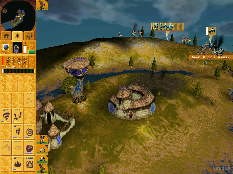
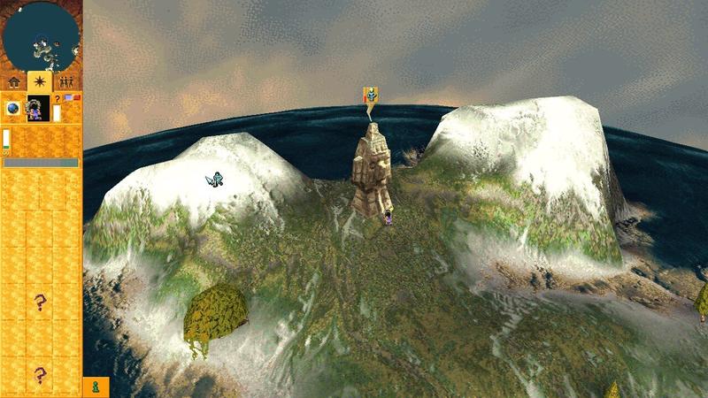
Populous: The Beginning is a strategy game released in 1998. The gameplay is fairly classic when you get down to it: across a series of levels, you grow your village and then go crush the rival tribes. This is largely thanks to the Shaman's powers, who unlocks new spells as the game progresses.

I was so fascinated by this game for two reasons, I think.

First, the terraforming possibilities were incredible: during a match, you could completely reshape the terrain through spells, building bridges, eroding the landscape, spawning volcanoes. It was pretty wild for the time.

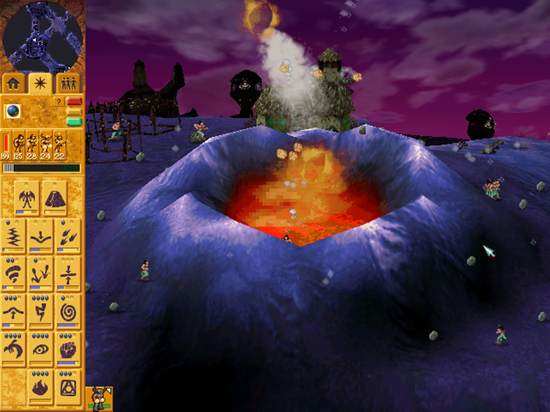
Most importantly, the graphics were incredible! Feast your eyes on these screenshots — which will probably make you chuckle a bit — but notice how the terrain feels alive. And above all, keep in mind that the rendering was entirely dynamic: you could throw a bridge between two hills, watch the terrain rise between them, and see the texture transform — shifting from a lush low-altitude meadow to rocky dirt to a snowy desert, all in real time.

3D low-poly pixel-art

I'm not the only 40-year-old developer letting nostalgia for the good old 640x480 games of my youth influence my work.

There's a whole movement of games going for a kind of "tribute" style that I'd call Low-poly Pixel-art.

A few examples will speak louder than words.

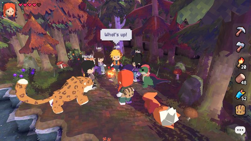
In short, the style is a blend of modern technique and retro influence. At high resolution, you apply deliberately pixelated texturing to simplified 3D models, sometimes mixing in 2D sprites.

Pixel-art in Rêvivarium

One of the challenges I had to tackle is that in Rêvivarium, the player can zoom all the way in to observe a blade of grass up close, or zoom all the way out to see the entire map.

One of the things that makes the style "work" is that the pixel density stays roughly constant on screen.

What you really want to avoid is one model with tiny pixels sitting next to another with pixels ten times larger.

So how do you guarantee the pixelated aesthetic holds up across all zoom levels?

In the rest of this article, we'll re-implement a 3D terrain in Godot, walking through the techniques I used.

Breaking down Populous's rendering

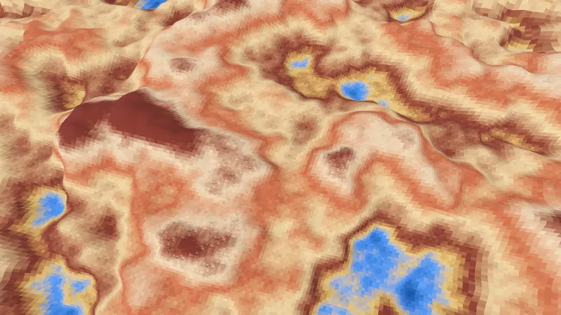
I spent a fair amount of time trying to figure out how Populous's rendering actually worked. At first glance, the principle relies on a very classic technique: a gradient maps a color to each elevation. But if that were all there was to it, the result wouldn't have the visual richness you'd expect.

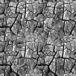
The heart of Populous's technique is the use of displacement textures that locally perturb the color selection. Two points at the same elevation can receive slightly different colors, which breaks up the flat bands and gives the terrain its pattern and visual richness.

This idea — an elevation gradient perturbed by a displacement map — is the foundation of our technique. The rest of the article tackles two problems: how to implement this rendering in a Godot shader, and how to pixelate it with a density that adapts to camera distance.

Laying the groundwork (pun intended)

We'll implement these techniques step by step in Godot. First up, let's create the object that will represent the terrain.

Note: I won't go into too much detail here since this step amounts to following the existing documentation.

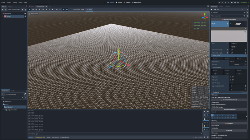
• create a new "Plane Mesh";
• set a size of 128x128 and a subdivision of 127x127;
• add a new material of type "Shader Material".

Note: I'll point you to Godot's excellent documentation on the topic if you're not sure what shaders are.

Setting up a basic render

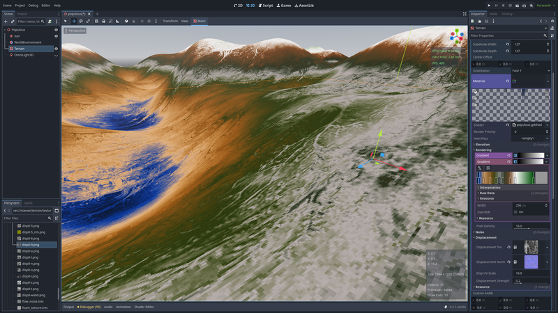
Let's implement an initial version with the core technique: a height map, a color gradient, and a displacement texture.

shader_type spatial;

group_uniforms World;
uniform vec2 world_size = vec2(128.0);  // Size of the terrain mesh

group_uniforms Elevation;
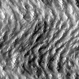
uniform sampler2D height_tex: hint_default_black, filter_linear_mipmap, repeat_disable;
uniform sampler2D normal_map_tex: hint_default_black, filter_linear_mipmap, repeat_disable;
uniform float height_max = 15.0;

group_uniforms Rendering;
uniform sampler2D gradient: source_color, filter_linear, repeat_disable;

group_uniforms Displacement;
uniform sampler2D displacement_tex: filter_linear_mipmap, repeat_enable;
uniform float displacement_strength: hint_range(0.0, 1.0) = 0.2;
uniform vec2 displacement_tex_size = vec2(4.0);  // World-space area one tile covers

void vertex() {
    // Sample the height texture to set the terrain topology
    float height = texture(height_tex, UV).r;
    VERTEX.y = height * height_max;
}

void fragment() {
    // Find base color depending on terrain height
    float height = texture(height_tex, UV).r;
    float color_index = height;

    // Add some texturing using the displacement map
    vec2 displacement_tiling = world_size / displacement_tex_size;
    vec2 displacement_uv = displacement_tiling * UV;
    float displacement = texture(displacement_tex, displacement_uv).r;

    // Use displacement to select the terrain color
    color_index += (displacement - 0.5) * displacement_strength;
    color_index = clamp(color_index, 0.0, 1.0);
    ALBEDO = texture(gradient, vec2(color_index, 0.0)).rgb;

    // Make sure lighting is correct
    vec3 normal = texture(normal_map_tex, UV).rgb;
    NORMAL_MAP = normal;
}

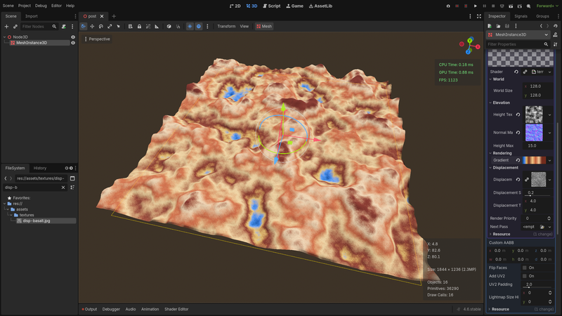
In the "Height Tex" field, create a new "NoiseTexture2D" and configure it to your liking. Make sure to check "Generate Mipmaps".

Then, drag and drop this texture into the "Normal Map Tex" field, open the menu next to the texture preview, and select "Make unique (recursive)" (otherwise the two textures can't be edited independently). Next, open the texture and click "As normal map".

For the color gradient, create a new "GradientTexture1D" and feel free to pick whatever color combination you like.

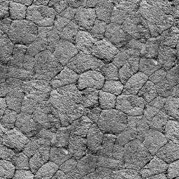
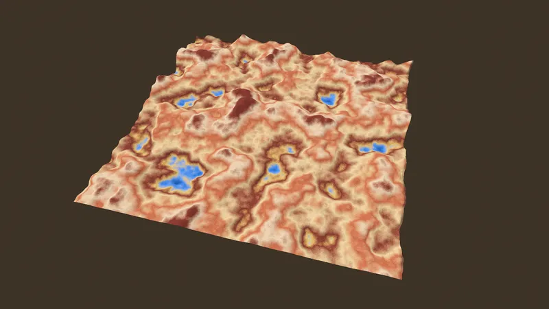
The "Displacement tex" is the texture that gives the terrain its pattern. You can use any tileable texture for this. For this tutorial, I used this one:

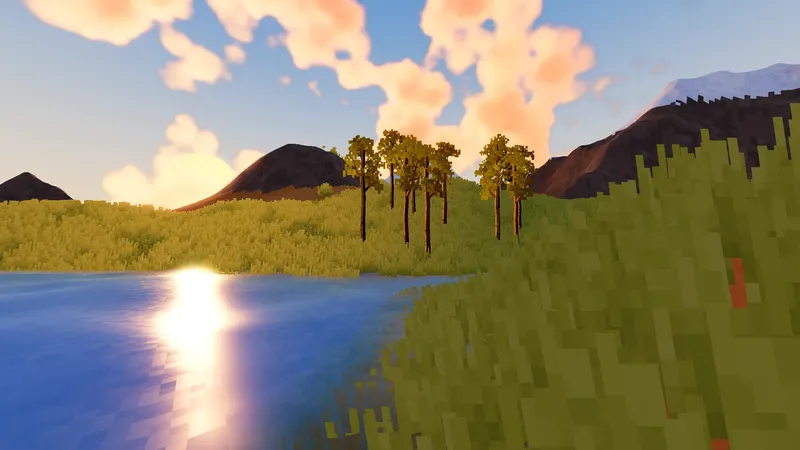
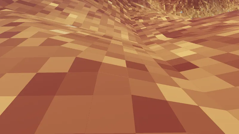
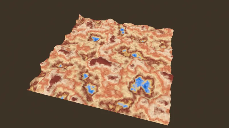
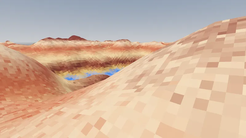
And you can admire the result of your work:

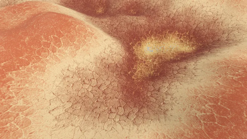
Zooming in close, you can see the rendering is perfectly smooth — a consequence of the linear interpolation declared on our textures.

Bring on the pixels

To get a pixelated look, let's add a new uniform to the shader:

uniform float pixel_density: hint_range(4.0, 32.0, 1.0) = 16.0;

This parameter lets us specify a grid of x pixels per meter on each side.

So if I have a 128m terrain and I want 16 pixels per linear meter (that's 16x16 = 256 pixels per square meter), that gives a total of 2048 pixels per side. All we need to do to make this grid real is to quantize the UV value.

Also, two things determine the terrain color: the elevation and the displacement map. We'll make sure to sample both values using the quantized UVs.

The relevant portion of the shader becomes:

// What is the width of the pixel-art grid?
vec2 grid_factor = world_size * pixel_density;

// Quantize the UVs
vec2 grid_uv = (floor(UV * grid_factor) + 0.5) / grid_factor;

// Add some texturing using the displacement map
vec2 displacement_tiling = world_size / displacement_tex_size;
vec2 displacement_uv = grid_uv * displacement_tiling;
float displacement = texture(displacement_tex, displacement_uv).r;

// Find base color depending on terrain height
float height = texture(height_tex, grid_uv).r;
…

Artifact problems and mipmaps

It's not very visible in the screenshots, but the current result has a very unpleasant problem.

The seams between pixels appear to have artifacts. You won't spot it in static screenshots, but when moving the camera, these seams produce a particularly maddening shimmer.

Explaining — and fixing — this problem requires a bit of a dive into how GPUs work.

Let's go back to our displacement texture declaration: filter_linear_mipmap. The linear flag tells the GPU to interpolate between texels — that's what produces the smooth look we saw up close. The mipmap flag enables automatic selection among several pre-computed versions of the texture at decreasing resolutions, known as mipmaps.

What are mipmaps? When a textured 3D model is seen from afar, multiple texels end up mapping to the same fragment — producing visual artifacts. Mipmaps solve this problem. When sampling, the GPU selects the right mipmap level based on texel density on screen [en].

So how does the GPU compute this density? It evaluates how quickly the UV changes from one fragment to the next. If the UV changes a lot between neighboring screen pixels, it means the texture is being viewed from far away, and a higher mipmap level can be selected.

When you sample a texture like this in the fragment shader:

float displacement = texture(displacement_tex, displacement_uv).r;

The GPU compares the current value of displacement_uv with the one computed by the neighboring fragment, and derives a mipmap level from that.

See the problem now? Since we've quantized the UV, the value is identical from one fragment to the next within each cell: the GPU thinks the texture is being viewed up close and selects a low mipmap. Then, at the boundary between cells, the sudden change causes the GPU to select a completely different mipmap right at the seam.

To fix the problem, two options: either we manually specify the desired mipmap using textureLod, or we compute the UV variation ourselves using textureGrad.

// Manually compute UV derivative for accurate mipmap selection
vec2 duvdx = dFdx(UV);
vec2 duvdy = dFdy(UV);

// Sample the displacement texture
float displacement = textureGrad(
    displacement_tex, displacement_uv,
    duvdx * displacement_tiling,
    duvdy * displacement_tiling).r;

// Find base color depending on terrain height
float height = textureGrad(height_tex, grid_uv, duvdx, duvdy).r;

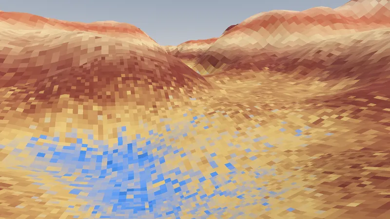
Who stole my pixels?

Let's pull back to survey our handiwork.

Damnatation 🏊! Who stole our pixels?!

The problem is that we introduced a pixelation tuned for a specific camera distance. From far away, our pixelated blocks get lost and simply become... pixels.

In a game where the camera stays at a roughly constant height, the previous technique can be enough. But if your game allows the camera distance to vary — and you want to maintain a pixelated aesthetic at all times — you'll need to get clever.

Let's look at solutions to this thorny problem.

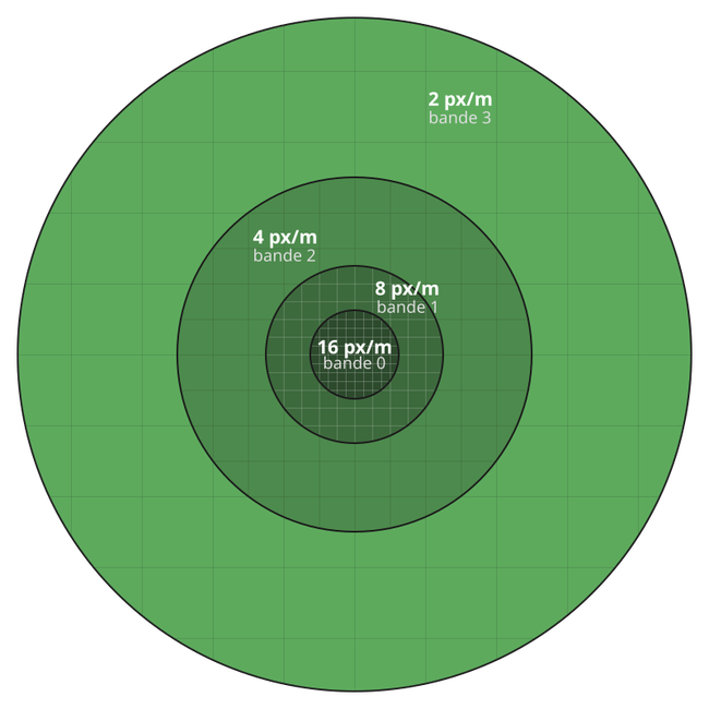
Adjusting density with distance

In a perspective projection, the linear size of an object on screen is inversely proportional to its distance.

Concretely, every time the distance between the object and the camera doubles, the side length of the area it occupies on screen is halved.

To maintain a roughly constant pixelation regardless of zoom level, we'll logically halve the pixel grid density when the distance doubles.

Computing fragment-to-camera distance

To compute the fragment-to-camera distance we need the camera's coordinates — which Godot helpfully provides — and the fragment's coordinates — which we don't have.

We'll need to retrieve them using a varying.

varying vec3 world_vertex;

void vertex() {
    …
    VERTEX.y = height * height_max;

    // VERTEX is in model coordinates, and we need world coordinates
    world_vertex = (MODEL_MATRIX * vec4(VERTEX, 1.0)).xyz;
}

void fragment() {
    float camera_dist = distance(CAMERA_POSITION_WORLD, world_vertex);
    …

Adjusting the density

We also want to make the reference distance — below which we keep the base density — configurable.

Let's add a new uniform:

uniform float pixel_reference_dist: hint_range(1.0, 50.0) = 5.0;

The function that increments each time its parameter doubles is log2.

void fragment() {
    float camera_dist = distance(CAMERA_POSITION_WORLD, world_vertex);

    // LOD band: increments each time camera distance doubles past min distance
    float lod = max(0.0, log2(camera_dist / pixel_reference_dist));
    float lod_band = floor(lod);

    // Halve density for each lod increment
    float band_density = pixel_density / exp2(lod_band);
    vec2 grid_factor = world_size * band_density;
    …

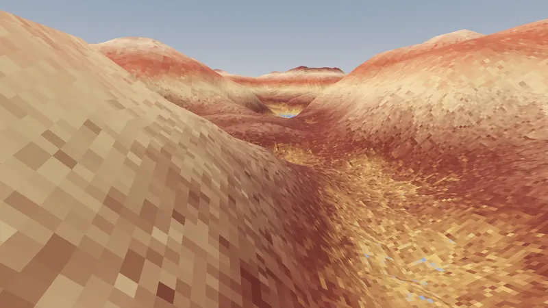
Let's admire the result.

Handling band transitions

You might think we're done, but not quite.

Our shader renders a continuous surface. The grid is pixelated, but the fragment-to-camera distance varies continuously: the switch from one density to the next happens without regard for any grid, creating inelegant "bands".

You have to look carefully to spot the problem in a still image, but when the camera is moving it's downright unbearable.

In pixel-art, cutting a pixel in half is a cardinal sin. So we need to replace this abrupt (and frankly ugly) transition with a progressive blending zone.

Notice that the two adjacent grids are aligned: the fine grid is a subdivision of the coarse grid, so each coarse pixel contains 2x2 = 4 fine pixels.

Our strategy: in the transition zone, we'll progressively "promote" fine-grid pixels to the coarse grid. The 4 adjacent fine pixels take on the coarse pixel's color one by one. By the end of the transition, every fine pixel has been promoted, and the coarse grid becomes the new fine grid for the next band.

Identifying the transition zone

Let's start by locating where these zones are. The fractional part of lod indicates the fragment's position within its band: 0 at the start, 1 just before the next band. We use it to create a transition ramp in the last band_transition_width percent of each band.

uniform float band_transition_width: hint_range(0.0, 0.5) = 0.3;

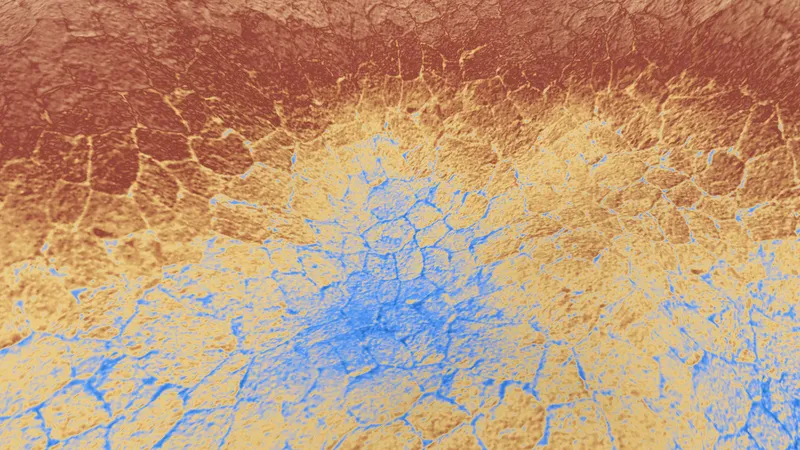
We temporarily replace the shader with a debug visualization.

void fragment() {
    float camera_dist = distance(CAMERA_POSITION_WORLD, world_vertex);
    float lod = max(0.0, log2(camera_dist / pixel_reference_dist));
    float transition = smoothstep(1.0 - band_transition_width, 1.0, fract(lod));

    // Debug: visualize the transition zones
    ALBEDO = vec3(transition);

Black means a fragment belongs to the core of a band; a black-to-white gradient marks the transition zone leading to the next band.

Promoting pixels

We compute both grids — fine and coarse — then, in the transition zone, we select one or the other for each fine pixel.

// Fine grid: snap UVs to the center of the current band's pixel cells
float density_fine = pixel_density / exp2(lod_band);
vec2 grid_factor_fine = world_size * density_fine;
ivec2 fine_cell = ivec2(floor(UV * grid_factor_fine));
vec2 grid_uv_fine = (vec2(fine_cell) + 0.5) / grid_factor_fine;

// Coarse grid: the next band's cells, at half the density
vec2 grid_factor_coarse = grid_factor_fine * 0.5;
vec2 grid_uv_coarse = (floor(UV * grid_factor_coarse) + 0.5) / grid_factor_coarse;

// Progressively promote fine pixels to the coarser grid
float transition = smoothstep(1.0 - band_transition_width, 1.0, fract(lod));
bool use_fine = ???
vec2 grid_uv = use_fine ? grid_uv_fine : grid_uv_coarse;

That leaves the central question: how do we choose which pixels to promote, and in what order?

Dithering and the Bayer matrix

Time to implement the last piece: the actual pixel selection for promotion.

Let's recap: for each fine pixel, we need a promotion threshold. In the transition zone, any pixel whose threshold is exceeded flips to the coarse grid.

A key requirement: promotions must be spatially dispersed — at any point during the transition, the pixels already promoted should be spread as uniformly as possible.

We could use a random value and cross our fingers, but there's a technique designed for exactly this: dithering (or "ordered dithering", to be precise).

Dithering is notably used to blend discrete values in a way that creates the perception of a smoother transition.

The technique could fill entire articles on its own [en] but that would be out of scope. The standard approach uses a Bayer matrix — a 2D array containing the promotion order for each position in the pattern.

The key property of this matrix: at every threshold, the cells already promoted are spread as uniformly as possible across the grid — that's what guarantees a visually smooth transition.

float bayer4x4(ivec2 cell) {
    int x = cell.x & 3;  // equivalent to % 4
    int y = cell.y & 3;
    mat4 m = mat4(
        vec4(0, 12, 3, 15),
        vec4(8, 4, 11, 7),
        vec4(2, 14, 1, 9),
        vec4(10, 6, 13, 5)
    );

    // Convert promotion order to transition threshold
    return (m[x][y] + 0.5) / 16.0;
}

The pattern repeats every 4 pixels. Each coarse pixel contains 2x2 = 4 fine pixels, and the 4x4 pattern spans 2x2 coarse pixels, which ensures variety both within and between neighboring pixels.

// Bayer dithered band transition. Each fine cell gets a fixed Bayer
// threshold. As fract(lod) nears 1.0, `transition` ramps up and cells
// whose threshold falls below it are promoted to the coarse grid.
float transition = smoothstep(1.0 - band_transition_width, 1.0, fract(lod));
float bayer = bayer4x4(fine_cell);
vec2 grid_uv = bayer > transition ? grid_uv_fine : grid_uv_coarse;

When transition is 0 (start of a band), all the Bayer thresholds are above it: every pixel stays on the fine grid. As transition increases, cells with the lowest thresholds get promoted first. When transition reaches 1, every pixel has flipped to the coarse grid, which in turn becomes the "fine" grid for the next band.

Complete shader

Here is the full implementation.

shader_type spatial;

group_uniforms World;
uniform vec2 world_size = vec2(128.0);  // Size of the terrain mesh

group_uniforms Elevation;
uniform sampler2D height_tex: hint_default_black, filter_linear_mipmap, repeat_disable;
uniform sampler2D normal_map_tex: hint_default_black, filter_linear_mipmap, repeat_disable;
uniform float height_max = 15.0;

group_uniforms Rendering;
uniform sampler2D gradient: source_color, filter_linear, repeat_disable;
uniform float pixel_density: hint_range(4.0, 32.0, 1.0) = 16.0;
uniform float pixel_reference_dist: hint_range(1.0, 50.0) = 8.0;
uniform float band_transition_width: hint_range(0.0, 0.5) = 0.3;

group_uniforms Displacement;
uniform sampler2D displacement_tex: filter_linear_mipmap, repeat_enable;
uniform float displacement_strength: hint_range(0.0, 1.0) = 0.2;
uniform vec2 displacement_tex_size = vec2(4.0);  // World-space area one tile covers

// Return a 4x4 Bayer matrix threshold for ordered dithering.
//
// Indexes the standard Bayer matrix by the low two bits of the cell
// coordinates, producing a spatially stable pattern tied to terrain pixels.
float bayer4x4(ivec2 cell) {
    int x = cell.x & 3;
    int y = cell.y & 3;
    mat4 m = mat4(
        vec4(0, 12, 3, 15),
        vec4(8, 4, 11, 7),
        vec4(2, 14, 1, 9),
        vec4(10, 6, 13, 5)
    );
    return (m[x][y] + 0.5) / 16.0;
}

varying vec3 world_vertex;

void vertex() {
    float height = texture(height_tex, UV).r;
    VERTEX.y = height * height_max;
    // Transform to world space for distance-based LOD in fragment()
    world_vertex = (MODEL_MATRIX * vec4(VERTEX, 1.0)).xyz;
}

void fragment() {
    // Per-fragment inputs. UV derivatives are captured before quantization:
    // quantized UVs are constant within each cell, so their screen-space
    // derivatives are zero — which would force the GPU to select mip 0.
    float camera_dist = distance(CAMERA_POSITION_WORLD, world_vertex);
    vec2 duvdx = dFdx(UV);
    vec2 duvdy = dFdy(UV);

    // LOD band: increments by one each time camera distance doubles past
    // the reference distance, halving pixel density at each step.
    float lod = max(0.0, log2(camera_dist / pixel_reference_dist));
    float lod_band = floor(lod);

    // Fine grid: snap UVs to the center of the current band's pixel cells.
    // grid_factor = total number of cells across the terrain.
    float density_fine = pixel_density / exp2(lod_band);
    vec2 grid_factor_fine = world_size * density_fine;
    ivec2 fine_cell = ivec2(floor(UV * grid_factor_fine));
    vec2 grid_uv_fine = (vec2(fine_cell) + 0.5) / grid_factor_fine;

    // Coarse grid: the next band's cells, at half the density.
    vec2 grid_factor_coarse = grid_factor_fine * 0.5;
    vec2 grid_uv_coarse = (floor(UV * grid_factor_coarse) + 0.5) / grid_factor_coarse;

    // Bayer dithered band transition. Each fine cell gets a fixed Bayer
    // threshold. As fract(lod) nears 1.0, `transition` ramps up and cells
    // whose threshold falls below it are promoted to the coarse grid.
    float transition = smoothstep(1.0 - band_transition_width, 1.0, fract(lod));
    float bayer = bayer4x4(fine_cell);
    vec2 grid_uv = bayer > transition ? grid_uv_fine : grid_uv_coarse;

    // Sample displacement texture, tiled across the terrain.
    // Derivatives are scaled by the tiling ratio (chain rule).
    vec2 displacement_tiling = world_size / displacement_tex_size;
    vec2 displacement_uv = grid_uv * displacement_tiling;
    vec2 disp_duvdx = duvdx * displacement_tiling;
    vec2 disp_duvdy = duvdy * displacement_tiling;
    float displacement = textureGrad(displacement_tex, displacement_uv, disp_duvdx, disp_duvdy).r;

    // Sample terrain height at the quantized position
    float height = textureGrad(height_tex, grid_uv, duvdx, duvdy).r;

    // Map height + displacement to a color via the gradient
    float color_index = height + (displacement - 0.5) * displacement_strength;
    color_index = clamp(color_index, 0.0, 1.0);
    ALBEDO = texture(gradient, vec2(color_index, 0.0)).rgb;

    NORMAL_MAP = texture(normal_map_tex, UV).rgb;
}

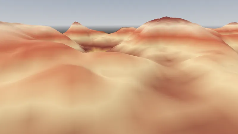
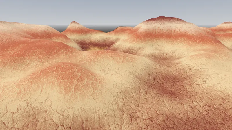
Final result

Populous's rendering felt alive because every pixel on the terrain contributed to the level's personality.

By combining the displacement map technique with adaptive pixelation — pixel density that varies with distance, and Bayer-matrix dithered transitions — we recapture that versatile, lively rendering that stays coherent at every scale.

These are two well-known techniques, but I'm not aware of any example where they've been combined. Am I about to become famous?

We could take this further: combining multiple materials, pixelating dynamic effects like flowing lava. But that'll be for another time.

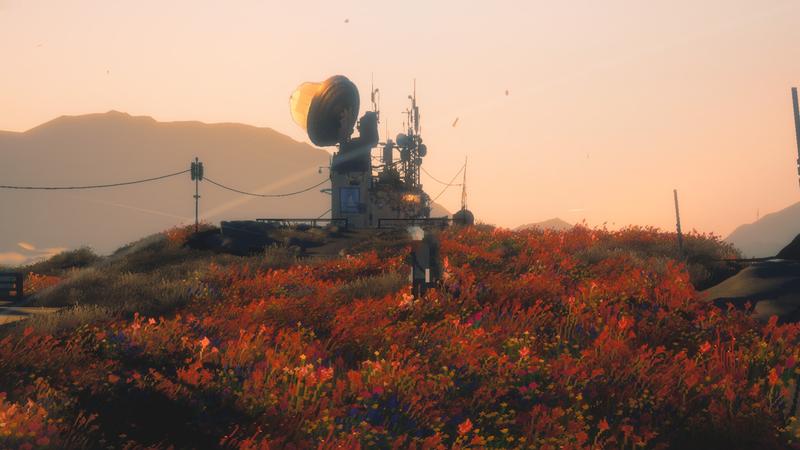
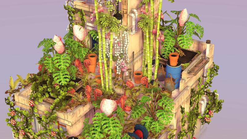
I'll leave you with a few examples from Rêvivarium.