Introduction to compute shaders with Godot
Modern games render staggeringly complex 3D environments, simulate entire cities teeming with life, or hordes of zombies charging at you. How do they harness the absurd power of today's hardware? With compute shaders.
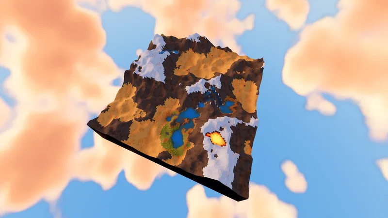
The first time I tried implementing a fluid simulation in GDScript, I got something that worked… at 3 fps.
A bit pathetic when you see some games simulating entire planets without breaking a sweat.
To get those results, you need the right tools. This article opens a series about compute shaders and how to use them with Godot.
Compute shaders are used extensively in Rêvivarium, and thanks to them, a whole living world is simulated in real time: water flows along the terrain and carves ravines, wind blows and carries sand into dunes, the sun heats the air, thousands of plants live and die according to their environment… All of it running on screen at 60 fps.
In this first installment, we will cover:
- what compute shaders are;
- how the cpu and the gpu interact;
- how to use compute shaders with Godot;
- a few essential principles and concepts.
Disclaimer: this post is a translation of the original french version.
Foreword
In a previous article, we discussed modern graphics architecture and the collaboration between CPU and GPU, which gave us a foundation for understanding vertex shaders and fragment shaders.
Compute shaders are not specific to Godot: every modern 3D graphics API (Vulkan, OpenGL, Metal, WebGPU…) provides compute shaders. Godot's job is to make these tools accessible through a unified interface.
In this article, we will try to cover both sides: the general principles that apply everywhere, and the Godot-specific implementation details.
Godot's documentation on compute shaders is quite sparse, amounting to little more than a quick introduction. While developing Rêvivarium, I ran into many practical situations where I had to figure things out on my own. This article comes from that experience and will go much further.
What is a compute shader?
Let's start with the basics.
A shader is a program that runs on the GPU (the graphics card).
Shaders are typically used for rendering:
- vertex shaders determine where on screen a 3D model should appear (for each vertex, a shader runs and computes the screen position);
- fragment shaders (sometimes pixel shaders) assign a pixel color to each fragment of the screen covered by said model.
Shaders are designed to run massively in parallel: thousands of instances of these programs run at the same time, each unaware of what the others are doing. It is this massive parallelism that delivers the real-time performance that makes video games possible.
A compute shader is the same thing, with one difference: it is not tied to a rendering task and can be used for any general-purpose computation.
So if I want to implement a feature that needs a large amount of computation, and those computations can run in parallel and independently of each other, compute shaders are the right tool:
- a fluid or particle simulation (each particle is independent);
- procedural texture generation (each pixel receives a value that depends only on its position in the grid);
- a physics simulation on a grid;
- computing the movement of thousands or millions of agents in a game;
- etc.
The cpu-gpu dance
The gpu is not a self-sufficient processor; the brain of the operation is still the cpu (in our case, a GDScript program).
It is the cpu that assigns tasks and commands the gpu to run shaders.
The interaction between the cpu and the gpu is fairly complex, and it took me a while to build a clear mental picture. So I am going to propose an analogy that we will carry through the article.
The cpu is a foreman with a mission: produce a succession of video game frames. He has a factory with an assembly line, but this factory can only work on one thing at a time. He also has a warehouse to store data (the RAM).
On the other side of town sits the gpu. It is a factory with hundreds or thousands of independent assembly lines, each operated by a specialized worker. These workers are extremely fast, but they can do nothing other than follow precise instructions (shaders). The gpu has its own memory warehouse (the VRAM).
The cpu and gpu each have a train station, connected by a rail line. Every frame, the foreman assembles a train made up of a series of wagons, each carrying execution orders or data.
The order we care about in this article has a name: the dispatch — "run this shader, on this data, this many times."
The train departs and reaches the gpu. A dispatcher walks through the wagons one by one, picks up the orders, and sets the assembly lines in motion. The specialized workers execute the orders to the letter, reading from and writing to the warehouse as they go.
When the work is done, the result is a complete frame sent straight to the display (no return trip to the cpu).
Sending a train is expensive (it requires a fair amount of OS-level and graphics-driver work), and it costs the same whether it carries one wagon or ten thousand. So the foreman's job is to prepare a full train so the entire frame can be built in one go, with no round trips. And the moment the train leaves, there is no downtime: the cpu immediately starts working on the next frame's train.
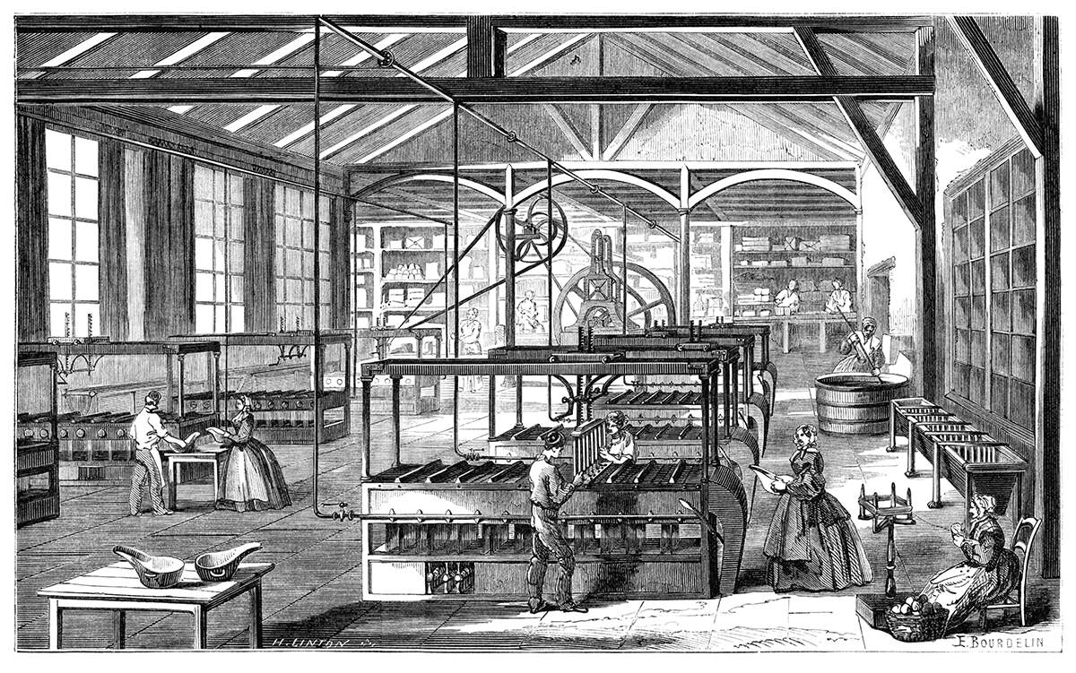
As you have gathered, the cpu cannot access the VRAM, just as the gpu cannot access the RAM. If the cpu wants to send data to the gpu, it must load it into a freight wagon. Conversely, if the cpu wants to read data from the gpu, it must send a wagon ordering the gpu to read the data and copy it into a freight wagon that will make the return trip.
Transferring data either way is therefore costly in time and bandwidth: the train has limited capacity, and overloading it means missing the deadline.
One last twist, and it is an important one: the gpu does not manage its own warehouse! That remains the foreman's job — he assigns and reserves memory locations. The gpu reads and writes data in the warehouse, but it is the cpu that keeps a ledger and is in charge of telling it what addresses to use for those reads and writes.
From this analogy, the key takeaways are:
- cpu and gpu are two distinct processing units;
- each has its own working memory;
- the cpu is in charge of everything and drives the operation;
- communication between cpu and gpu is heavily asynchronous — when an order leaves, it can take 2 or 3 frames before the result shows up;
- data transfer and bandwidth are critically important.
A first shader
Enough analogies — here is a shader as concrete as it gets.
The following shader "paints an image" with a single color: it receives an image and a color as inputs, and writes that color into every pixel of the image.
#[compute]
#version 450

// The GPU runs this program in workgroups of 8x8 invocations.
layout(local_size_x = 8, local_size_y = 8, local_size_z = 1) in;

// The texture we write into: four float channels per texel.
layout(set = 0, binding = 0, rgba32f) uniform restrict writeonly image2D color_out;

// The parameters sent along with each dispatch.
layout(push_constant, std430) uniform Params {
    vec4 color;
} params;

void main() {
    // This invocation's number in the dispatch is also the texel it handles.
    ivec2 texel = ivec2(gl_GlobalInvocationID.xy);
    imageStore(color_out, texel, params.color);
}
Let's break it down.
#[compute]
This line is a Godot-specific marker that tells the engine this file contains a compute shader.
#version 450
Several languages exist for programming shaders, each with multiple versions. Godot expects GLSL code, version 450.
layout…
The next three lines start with layout, a keyword that is not an instruction but an annotation. layout configures the declaration that follows it. To read a layout line, it is easier to start from the end.
// The GPU runs this program in workgroups of 8x8 invocations.
layout(local_size_x = 8, local_size_y = 8, local_size_z = 1) in;
Here the declaration says nothing more than that it is an input parameter (in), applying to the program itself. This line tells the GPU that the shader will be launched in parallel groups of 64 executions. The concepts of invocation and workgroup are essential and will be explained right after the code.
// The texture we write into: four float channels per texel.
layout(set = 0, binding = 0, rgba32f) uniform restrict writeonly image2D color_out;
To understand this line, we read from the end.
color_out: we declare a variable…image2D: …of typeimage2D, a two-dimensional image that the shader can access pixel by pixel, like a raw two-dimensional array.restrictandwriteonly: we declare that this variable will be written and not read, and that no other variable will access the same memory region. These are optional hints that let the gpu optimize performance.uniform: the variable comes from the outside and will be provided by the cpu; "uniform" because every invocation of the shader will receive exactly the same variable.
Then comes the layout annotation:
set = 0, binding = 0: the shader needs to work with an image stored in memory, but where? As we said, it is the cpu that keeps the gpu's warehouse ledger.
So the shader declares "I will look up this image's address on supply slip 0, line 0." It is the cpu that will fill in this supply slip before the train departs — we will see how in detail.
rgba32f: tells the gpu the format of the image's pixels. Here, four channels (rgba), each value stored as a 32-bit float.
// The parameters sent along with each dispatch.
layout(push_constant, std430) uniform Params {
    vec4 color;
} params;
params: the name of the variable.Params { vec4 color; }: we define a struct (a group of fields) containing a single fieldcolorof typevec4.uniform: as with the image, it is the cpu that will provide the value, identical for all invocations.
The layout here needs some explanation.
push_constant: the cpu has several ways to pass values to the gpu that will run the shader.
Heavy data travels in freight wagons and stays in the gpu's warehouse. But you often need to pass the shader a few parameters that change with every dispatch. For that, you use push constants: a handful of bytes pinned to the work order itself — they travel with the order, no freight wagon needed.
std430: when it receives an execution command, the gpu knows where the data sits in memory, but not exactly how it is laid out. Which byte corresponds to which variable? The cpu and gpu must agree on how data is packed and decoded, because multiple conventions exist. std430 is one of them. I will not go into more detail for now — it is a real can of worms that will get its own treatment in another article.
void main() {
The shader's main entry point.
// This invocation's number in the dispatch is also the texel it handles.
ivec2 texel = ivec2(gl_GlobalInvocationID.xy);
As we are about to see, the shader runs in many simultaneous invocations. To tell them apart, each invocation receives parameters that identify its position within the overall computation.
Here I will arrange for the total number of invocations to match the number of pixels in the image I am working on (say 512 x 512). So this shader is written to treat its unique invocation number gl_GlobalInvocationID.xy as exact coordinates in the pixel grid.
We will come back to this right after.
imageStore(color_out, texel, params.color);
We call a native GLSL function that assigns a color to a pixel by writing a value to the appropriate memory location.
What to take away from this first shader:
- the shader specifies which supply slip (set, binding) the cpu must fill in so it knows the memory address of a variable;
- it also specifies the expected data format;
- the cpu must follow these instructions when preparing the dispatch.
Invocations and workgroups
The shader above paints an entire image with a given color: every pixel of the image will receive the color passed as a parameter.
If we had wanted to write such a function in another language, we would probably have used a loop. In pseudocode:
for x in 0 to image_width:
  for y in 0 to image_height:
    image.writePixel(x, y, color)
But you may have noticed there is no loop in this shader — just a single imageStore instruction writing one pixel at one address.
This is where the shift in mindset happens: a shader is one program run a large number of times. Each instance must carry out a fraction of the total work independently.
Which brings us back to the absolutely essential concepts of invocations and workgroups.
An invocation is a single execution of a shader. If your shader writes one pixel and you have ten invocations, you will write ten pixels.
GPUs never launch a single invocation — that would defeat the whole point of parallelism. Shaders run in fixed-size groups called workgroups, and it is the shader itself that declares the group size.
Say I want to run an operation on a 512x512 pixel texture. I know the shader declares a workgroup of 8x8, so each workgroup will handle an 8x8 block of pixels. To cover the entire texture, the cpu must therefore dispatch 64 x 64 workgroups (512 / 8 = 64 on each axis).
The total number of invocations will be 64 x 64 x 8 x 8 = 262,144 — the number of pixels in the texture.
And yes, this total is configured in two parts:
- the workgroup size (set in the shader);
- multiplied by the number of workgroups dispatched (set in GDScript).
You can now decode the name gl_GlobalInvocationID: this invocation's number within the global computation, across all workgroups. It is exactly the unique value, between 0 and 511 on each axis, that each invocation of our first shader received.
The companion project
Throughout this series of articles, we will build a simulation with Godot, inspired by Rêvivarium: an island with water flowing down its slopes, a few physical phenomena — all in real time.
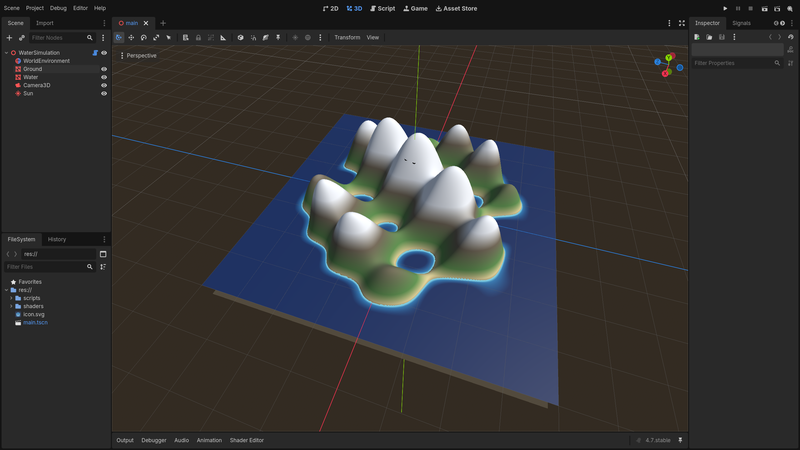
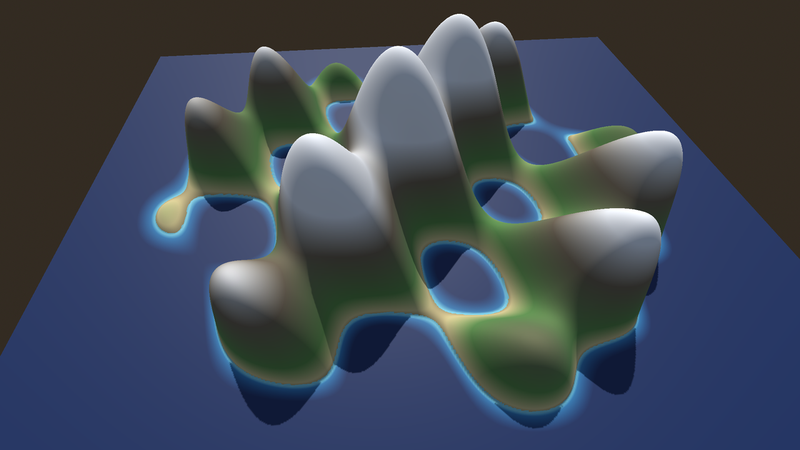
Here is what we are going to build in this first installment: a Godot project with two planes, one representing the terrain, the other the water. The height data will be stored in a texture, initialized by a compute shader.
I will assume a basic familiarity with Godot, so the following steps will not be overly detailed.
Start a new Godot project and set up the scene tree as follows:
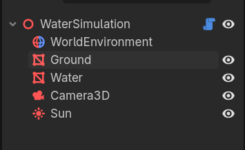
Ground and Water are two meshes that will represent the terrain and the flowing water. To set them up, create two MeshInstance3D nodes, assign each a new PlaneMesh, set the size to 512m, and the subdivision to 511. Assign each mesh a ShaderMaterial and create two Godot shaders, ground.gdshader and water.gdshader.
These two shaders work in a similar way: they read a height value from a texture, displace the mesh accordingly, and assign each fragment a color based on its altitude.
For now this is very similar to what you will find in the official Godot documentation or in this earlier post about pixel-art terrain.
The code for ground.gdshader:
shader_type spatial;

// Renders the terrain: vertices displaced by the terrain height, colors
// from an altitude gradient.

// The texture that holds the heightmap data
uniform sampler2D world_tex : filter_linear, repeat_disable;

// A gradient: altitude -> color
uniform sampler2D gradient : source_color, filter_linear, repeat_disable;

// Altitude covered by each half of the gradient: the gradient spans
// [-max_height, +max_height] around sea level.
uniform float max_height = 100.0;

// Terrain height at a texture coordinate, in world units (0 = sea level).
float height_at(vec2 uv) {
    return texture(world_tex, uv).r;
}

// Surface normal at a texture coordinate
// Compute the normal vector dynamically, so the lighting is correct
// This is out of scope for the content of this post, you can safely
// ignore that method.
vec3 normal_at(vec2 uv) {
    vec2 texel = 1.0 / vec2(textureSize(world_tex, 0));
    float height = height_at(uv);
    float height_right = height_at(uv + vec2(texel.x, 0.0));
    float height_down = height_at(uv + vec2(0.0, texel.y));
    vec3 right = vec3(1.0, height_right - height, 0.0);
    vec3 down = vec3(0.0, height_down - height, 1.0);
    return normalize(cross(down, right));
}

void vertex() {
    // Set up the terrain mesh from the heightmap texture
    // Update each vertex vertical coordinates
    // using data from the world texture
    VERTEX.y += height_at(UV);
    NORMAL = normal_at(UV);
}

void fragment() {
    // Find the terrain color from altitude -> gradient
    float gradient_position = height_at(UV) / (2.0 * max_height) + 0.5;
    ALBEDO = texture(gradient, vec2(gradient_position, 0.0)).rgb;
    ROUGHNESS = 1.0;
}
water.gdshader:
shader_type spatial;

// Renders the water surface: vertices displaced to the top of the water
// column (terrain height + water depth), colors from a depth gradient.

uniform sampler2D world_tex : filter_linear, repeat_disable;
uniform sampler2D depth_gradient : source_color, filter_linear, repeat_disable;

// Water depth that reaches the darkest end of the gradient.
uniform float max_depth = 20.0;

// Where the depth is zero, the water surface would coincide exactly with
// the terrain and the two would flicker (z-fighting).
// Sinking the water a bit lower hides dry areas below the terrain.
const float DRY_OFFSET = 0.05;

// Water surface height at a texture coordinate: the terrain plus the
// water sitting on it, in world units.
float surface_at(vec2 uv) {
    vec2 world = texture(world_tex, uv).rg;
    return world.r + world.g;
}

// Surface normal at a texture coordinate
vec3 normal_at(vec2 uv) {
    vec2 texel = 1.0 / vec2(textureSize(world_tex, 0));
    float height = surface_at(uv);
    float height_right = surface_at(uv + vec2(texel.x, 0.0));
    float height_down = surface_at(uv + vec2(0.0, texel.y));
    vec3 right = vec3(1.0, height_right - height, 0.0);
    vec3 down = vec3(0.0, height_down - height, 1.0);
    return normalize(cross(down, right));
}

void vertex() {
    VERTEX.y += surface_at(UV) - DRY_OFFSET;
    NORMAL = normal_at(UV);
}

void fragment() {
    float water_depth = texture(world_tex, UV).g;
    float gradient_position = min(water_depth / max_depth, 1.0);
    ALBEDO = texture(depth_gradient, vec2(gradient_position, 0.0)).rgb;
    ROUGHNESS = 0.6;
}
In these two shaders, we declare three uniforms that need to be configured: gradient, depth_gradient, and world_tex.
In the Godot inspector, you can manually set up the two gradients with whatever colors inspire you.
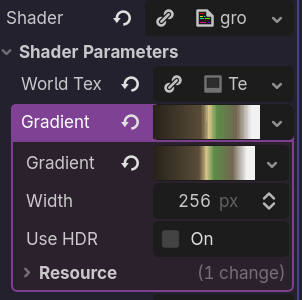
That leaves the world_tex texture: it needs two channels (r, g), each holding a height value — r for the terrain height, g for the water depth. This texture does not exist yet. We will fix that in the next step.
Initializing the heightmap
Attach a script to the root WaterSimulation node. Here is the code for the new water_simulation.gd:
@tool
extends Node3D
## Runs the water simulation on the GPU and displays the result.

# The size of the world and texture we want
const GRID_SIZE := 512

# The workgroup defined in the shader
const WORKGROUP_SIZE := 8

@onready var ground: MeshInstance3D = $Ground
@onready var water: MeshInstance3D = $Water

# The RenderingDevice is a Godot server: a low-level api that gives
# direct access to graphic APIs
# See https://docs.godotengine.org/en/stable/classes/class_renderingdevice.html
# and https://docs.godotengine.org/en/stable/tutorials/performance/using_servers.html
var rd: RenderingDevice

# Those are the resources we need to compile and run the shader
# RIDs are entries in the gpu memory registry the cpu maintains.
# We'll get back to it later.
var shader: RID
var pipeline: RID

# The whole world lives in this GPU texture
# We decide that one texel = one cell of the grid = one m²
# red channel = terrain height, green channel = water depth.
var world_texture: RID

# The world texture will only live on the gpu.
# Current code lives on the cpu.
# Godot provides a special texture type Texture2DRD that bridges the two.
# I can pass this texture to a Godot material that will access the data
# directly on the gpu.
var world_texture_display: Texture2DRD


func _ready() -> void:
    world_texture_display = Texture2DRD.new()

    # Pass the Texture2DRD reference to the shaders
    ground.mesh.material.set_shader_parameter("world_tex", world_texture_display)
    water.mesh.material.set_shader_parameter("world_tex", world_texture_display)

    # Every gpu-related operation must originate from the rendering thread
    RenderingServer.call_on_render_thread(init_gpu)


## Create the GPU resources, generate the island, connect the display.
func init_gpu() -> void:
    rd = RenderingServer.get_rendering_device()

    create_world_texture()
    create_island_pipeline()
    generate_island()

    # Here we bind a Godot classical 2d texture to actual data on the gpu
    world_texture_display.texture_rd_rid = world_texture


## Create the texture in the gpu memory
# Well, not really...
# We are only creating a new entry in the cpu registry.
# The cpu now knows that there is one allocated block in the
# gpu memory at a specific address, made to hold data with
# specific image characteristics.
# Nothing happens in memory yet, and the actual data is simply garbage.
func create_world_texture() -> void:

    # First setup the texture characteristics
    # Provide the size (width / height) and format (two 32-bit float channels)
    var format := RDTextureFormat.new()
    format.width = GRID_SIZE
    format.height = GRID_SIZE
    format.format = RenderingDevice.DATA_FORMAT_R32G32_SFLOAT

    # The format can take some flags that will configure
    # different permissions.
    #  - our compute shader will write into it
    #  - the display materials will read it
    #  - the Godot editor will read it back to draw inspector previews.
    format.usage_bits = (
        RenderingDevice.TEXTURE_USAGE_STORAGE_BIT |
        RenderingDevice.TEXTURE_USAGE_SAMPLING_BIT |
        RenderingDevice.TEXTURE_USAGE_CAN_COPY_FROM_BIT
    )

    # Delegate to the graphics API the texture creation
    world_texture = rd.texture_create(format, RDTextureView.new())


## Load and compile the shader
func create_island_pipeline() -> void:
    var shader_file: RDShaderFile = load("res://shaders/generate_island.glsl")
    shader = rd.shader_create_from_spirv(shader_file.get_spirv())
    pipeline = rd.compute_pipeline_create(shader)


## Ask the GPU to run the island generation shader
func generate_island() -> void:
    # This operation gives the shader access to the texture.
    # A uniform set is a supply slip: numbered lines, each naming a
    # resource from the warehouse. Here: line 0 of slip 0 names our
    # world texture.
    var uniform := RDUniform.new()
    uniform.uniform_type = RenderingDevice.UNIFORM_TYPE_IMAGE
    uniform.binding = 0
    uniform.add_id(world_texture)
    var uniform_set := rd.uniform_set_create([uniform], shader, 0)

    # Initialize the push constant.
    # The shader will receive it in its `params` variable.
    # For technical and obscure (for now) reasons, the block size
    # must be a multiple of 16 bytes.
    var params := PackedFloat32Array([GRID_SIZE, GRID_SIZE, 0.0, 0.0])
    var push_constant := params.to_byte_array()

    # 512 cells wide / 8 invocations per workgroup = 64 workgroups per axis.
    # Right now, the texture size is a multiple of the workgroup size,
    # so no invocation will be "wasted", but that shall not always be the
    # case.
    var groups := ceili(float(GRID_SIZE) / WORKGROUP_SIZE)

    # A Compute List holds a series of gpu instructions.
    # It's like a single wagon of the "train of commands" the cpu
    # is building, but a wagon in itself can hold several instructions.
    # When it receives them, the gpu will execute them in order.

    # So don't see this as "execute this shader", rather "add this
    # to the list of instructions the cpu is preparing to send
    # to the gpu to build the entire frame".
    var compute_list := rd.compute_list_begin()

    # Tells the gpu "from now on, the loaded program is this one"
    rd.compute_list_bind_compute_pipeline(compute_list, pipeline)

    # Hand the supply slip to the crews
    rd.compute_list_bind_uniform_set(compute_list, uniform_set, 0)

    # Set up the push constant
    rd.compute_list_set_push_constant(
        compute_list, push_constant, push_constant.size())

    # Add a dispatch to the list of commands
    rd.compute_list_dispatch(compute_list, groups, groups, 1)

    # We could add several dispatches in a single compute list
    # but for now we only need one.
    rd.compute_list_end()
The script is heavily commented. A few points still deserve some clarification.
A low-level API
RenderingDevice is a very low-level API — almost no abstraction. It is essentially a thin wrapper over the underlying graphics API (Vulkan, Direct3D 12, Metal…).
As a result, the Godot-specific part stops here: the shader that follows is standard GLSL, which would work identically in any engine.
Rendering devices, compute lists, and wagons
If you have read the docs, you may have seen that Godot distinguishes between the global rendering device and local rendering devices. As we explained, Godot builds — for each frame — a command train that it sends to the gpu. When you write the following code…
rd = RenderingServer.get_rendering_device()
…
rd.compute_list_begin()
…you are adding your own wagon to the existing train, and you are bound by its schedule. You do not decide when the train leaves — Godot does — and you cannot wait for it to arrive: by the time the gpu executes your commands, Godot has already moved on to the next frames. You cannot block everything to wait for a result, because that would block the entire rendering pipeline for milliseconds.
The official documentation uses local rendering devices. This amounts to opening your own private line to the gpu, with your own trains that you manage as you please: you can dispatch a shader, wait for the result — all without blocking the main display. It has its uses and its constraints, but it is out of scope for now. Knowing the difference exists is useful for making sense of the Godot docs.
The rendering thread
In Godot, rendering code runs in a dedicated thread (if the corresponding option is enabled) — a thread on the cpu, to be clear.
As a rule, every call to the rendering API (RenderingDevice) must happen on that thread. That is why we use call_on_render_thread.
Shaders, pipelines, and compilation
A word about shader compilation and the shader/pipeline distinction.
You write a shader in GLSL — it is a text file. This text is transformed into an intermediate format — SPIR-V (which we do not really need to worry about) — that is not executable as-is.
A further transformation is needed: the actual compilation that produces executable code. The final result is the pipeline. Pipeline = compiled program. Why this name? It comes from the graphics side, where the pipeline refers to the chain of stages that vertices pass through (vertex shader, rasterizer, fragment shader…).
Why are these two steps necessary? That is a topic in its own right, which will be covered in another article in the series.
Resource lifecycle
The cpu reserves space in the gpu's memory, but that memory is never freed.
As it stands, our current code contains lovely memory leaks.
Resource lifecycle is a topic that deserves its own treatment, and we will cover it in more detail in the next article of the series.
The shader at last
And now, the shader code:
#[compute]
#version 450

// Generate the island terrain and its initial sea.
//
// One invocation runs per cell and writes that cell's terrain height (red
// channel) and water depth (green channel). One cell spans one world unit;
// heights are world units too, and 0 is the sea level.

// The GPU runs this program in workgroups of 8x8 invocations.
layout(local_size_x = 8, local_size_y = 8, local_size_z = 1) in;

// The texture we write the world into. "rg32f" = two float channels per
// texel. The GDScript side attaches the texture here (set 0, binding 0).
layout(set = 0, binding = 0, rg32f) uniform restrict writeonly image2D world_out;

// The parameters the GDScript side sends along with each dispatch.
layout(push_constant, std430) uniform Params {
    vec2 grid_size;
    vec2 _pad; // unused, rounds the block size up to 16 bytes
} params;

// Depth of the open sea around the island, in world units.
const float SEA_DEPTH = 45.0;

const float PI = 3.14159265;

// Terrain height at a position of the map (both axes from 0 to 1), in
// world units, 0 at sea level.
// Feel free to treat it as a black box and skip ahead.
// Or replace it with whatever funky heightmap generation
// code you want.
float island_height(vec2 uv) {
    // How far this position is from the center of the map: 0 at the
    // center, 1 at the middle of the map borders.
    float distance_to_center = length(uv - 0.5) * 2.0;

    // The island silhouette: 1 at the center, fading to 0 between 55% and
    // 95% of the way out — so open sea surrounds the land.
    float island_shape = 1.0 - smoothstep(0.55, 0.95, distance_to_center);

    // The land, made of overlapping waves of different sizes, in world
    // units: a 100-unit dome peaking at the center of the map, hills half
    // as tall, bumps half as tall again. The hill and bump frequencies are
    // arbitrary — change them, the island changes.
    float dome = sin(uv.x * PI) * sin(uv.y * PI) * 100.0;
    float hills = sin(uv.x * 17.0 + uv.y * 12.0) * 50.0;
    float bumps = sin(uv.x * 31.0 - uv.y * 27.0) * 25.0;
    float land = (dome + hills + bumps) * island_shape;

    // Sink everything: where the island faded to nothing, only the open
    // sea floor remains.
    return land - SEA_DEPTH;
}

void main() {
    // Invocation number = coordinates of the terrain cell it handles
    ivec2 cell = ivec2(gl_GlobalInvocationID.xy);

    // Sometimes, we can't get exactly the number of invocation we want.
    // If workgroup size is 8x8, the total invocation count will be a multiple of that.
    // If the texture does not match those dimensions, then some invocations will
    // "overshoot" so we have to add a guard clause.
    ivec2 size = ivec2(params.grid_size);
    if (cell.x >= size.x || cell.y >= size.y) {
        return;
    }

    // Normalizes grid-sized coordinates (0 to grid_size) to [0;1] coordinates.
    // (+0.5 targets the center of the cell).
    vec2 uv = (vec2(cell) + 0.5) / params.grid_size;

    // Find the terrain height at those coordinates
    float height = island_height(uv);

    // The sea fills everything below zero.
    float water = max(0.0, -height);

    // imageStore always takes a vec4.
    // Our texture only keeps the first two channels and drops the rest.
    imageStore(world_out, cell, vec4(height, water, 0.0, 0.0));
}
If you have followed the instructions to the letter, reload the scene and an island should appear in your editor.
Conclusion
We have started using compute shaders in a simple case, explored how the cpu and the gpu communicate, and laid out the principles and pitfalls we will need to keep in mind.
So far, here is what we have built:
A Godot scene tree with an initialization script. This script creates a texture in memory. It calls a compute shader that fills the texture with height data. It also passes a reference to the terrain and water display shaders so they can access the data.
The beauty of this system is that it is extremely fast. The cpu has very little to do: it reserves a memory block, prepares a dispatch, sends it off to the gpu, and calls it a day. The gpu initializes the texture and the gpu handles the display.
And the best part: the data stays on the gpu. As things stand, the cpu has no access to the data — there has been no memory transfer, not a single freight wagon has traveled. We could have pulled the data back to the cpu and re-uploaded it to the Godot shaders, but that would have been a costly and pointless round trip.
In the rest of the series, we will keep building on our island, each new addition exploring new concepts and techniques.